Congestion control

Congestion control has become a fundamental guiding principle in designing end-to-end Internet protocols, and is necessary for the communication to work. In this module we

Remind ourselves about the traditional principles of congestion control, which likely is familiar from a basic computer networks course earlier.
Discuss buffering in the network, and the latency and reduced user experience it causes. In today’s networks network latency is a key quality criteria. We also discuss ways to reduce the latency in the network.
Get familiar with Explicit Congestion Notification (ECN), that is a protocol for the network to signal congestion to the end hosts, that can then try to avoid congestion early on.
Discuss different types of modern congestion control algorithms that have emerged since the original algorithm, and are widely used in current system implementations.

Related assignment: Data transfer using UDP

Traditional congestion control

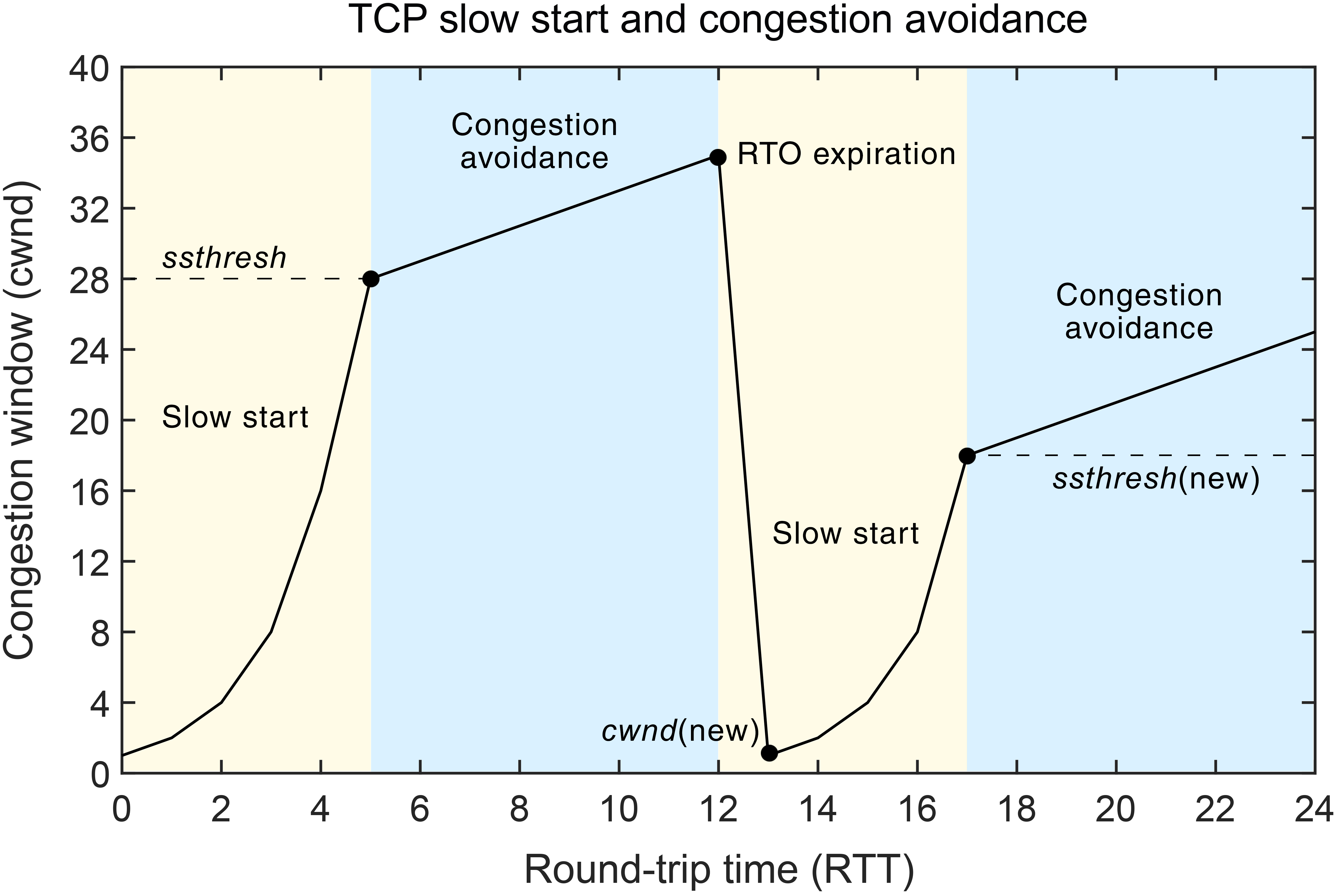
The fundamental principles of congestion control were introduced in the classic paper by Van Jacobson, when first congestion collapses were detected in TCP communication in the 1980s. The paper introduced the slow-start strategy, where at the beginning of TCP connection, or after retransmission timeout, the congestion window size is increased by the size of one segment for each incoming acknowledgment, i.e. effectively causing the window size to double every round-trip time (RTT). RTT is the time it takes from sending a data packet until the acknowledgment for the data comes back. This is one of the most important metrics in any congestion control algorithm, and in analysis of end-to-end performance. Congestion window indicates how many segments (or full-sized packets) can be in transit at the same time before acknowledgment for the first packet comes in.

The paper also introduced congestion avoidance algorithm, where the congestion window is increased by $1/cwnd$ for each acknowledged segment. In other words, congestion window is increased by one segment each round-trip time. Congestion avoidance is applied when congestion window exceeds the slow-start threshold, that indicates the number of unacknowledged segments at the time the last loss event occurred.

The following graph from encyclopedia.pub illustrates TCP’s slow start and congestion avoidance, a behavior that is probably well-known from earlier computer network courses.

The paper also discusses packet conservation principle, the idea that transmission of new data should only be triggered when an acknowledgment arrives. This self-clocking property causes the transmission of packets to be paced by the actual network round-trip time. If the round-trip time increases for some reason in the middle of transmit, also the packet transmission reacts accordingly.

The idea of early congestion control until these days has been, that packet loss is most likely caused by a full buffer at some network device along the way, i.e., caused by a congestion where transmission rate exceeds the network’s capacity to delivery of packets. While this is often true, there are special networks, particularly wireless networks, where packet loss can also be caused by a corruption of packet because of poor transmission link, which is detected by the receiver because through faulty checksum. Packet loss is often also too slow signal for timely congestion reaction, because it arrives one round-trip time “too late”. As we will see shortly, this may cause poor performance in data transmission, especially when packet are transmitted fast but delay of propagating the packet takes proportionally long. Therefore much research to improve congestion control has been done over the years until the recent days.

Network buffering and latency

The network devices have buffers and queues for packets waiting to be sent, and for incoming packets waiting to be processed. Almost certainly there will be a point in the network path where the network device is not able to transmit packets out as fast as they arrive. Possible reason is, for example, that the outgoing link technology has less bandwidth for transmitting data, than what the incoming links have. This may happen, for example, in some wireless technologies, or slow home network service. Other common reason is, that there are multiple incoming packet sources that are to be forwarded to a shared link.

When packet queue reaches its capacity, it cannot take more packets and packet loss results. Eventually, roughly one round-trip time later, the original sender of the packet notices the packet signal, for example from consecutive incoming duplicate acknowledgments missing the lost packet, or from retransmission timeout, if no more acknowledgments arrive. Before the packet queue gets full it may have received multiple, some times large number of packets that are still waiting in the queue for transmission.

The end-to-end round-trip delay does not only consist of delay of data transmission at sending device, or the propagation of bits over link, even though that would be an ideal situation. In many situations large portion of end-to-end delay is due to packet waiting in network queue. Some network device operators try to maintain fairly large queues to avoid packet losses in bursty traffic patterns. Therefore also the end-to-end delays and data delivery latency increase. With some traditional network applications (e.g., file transfer) this may have been acceptable trade-off. However, many of today’s network applications, such as online games or interactive voice/video calls or even the modern interactive web pages are more sensitive to delay that causes bad user experience for the end users.

Term “Bufferbloat” was invented for the issue of network overbuffering and resulting negative effects. The question is, what should be the correct size of buffers and queues at each network device, when typically each connection traverses multiple switches and routers between sender and receiver? It is known that network traffic arrives in bursty patterns, partially because of the operation logic of many network applications (such as web browsing), and partially how the traditional TCP congestion control works, especially in slow-start. Longer buffers help to absorb such bursts without packet losses, at the cost of increased delays.

The below graph, from a network article “Buffer-Bloated Router? How to Prevent It and Improve Performance” in the Communications of the ACM, illustrates the development of network throughput and experience delay as the function of rate of packets transmitted over network. The vertical line illustrates the point where the outgoing link can absorb all data it receives without needing to queue data. One can see the tradeoff congestion control algorithms are trying to solve: if the transmission rate (or congestion window) is too small, then the available network throughput is not fully utilized, even though delay is stable, as determined by propagation of bits. If the transmission rate is too high, we do not gain anything in throughput, because the outgoing link is fully utilized, but delay increases as packets are buffered.

Active Queue Management

The traditional tail-drop queue behavior has a couple of particular problems. The window-based congestion control and the network traffic patterns tend to cause some of the non-real time traffic flows to be bursty. When such burst arrives at a full queue, several packets from that flow will be dropped. Therefore the losses can be unevenly split between flows, biasing against bursty traffic. The other problem relates to the delay in receiving congestion signal at the sender. When the queue is full and packets get dropped from multiple flows, then all flows react by reducing transmission rate, which causes the overall throughput to drop excessively for a moment due to this synchronized effect, until congestion windows at different senders start to increase again.

Active queue management algorithms aim to control the queue length before it gets full, and incoming packets must be dropped. If the transport protocol supports explicit congestion notification, together with active queue management the data sender can be asked to slow down transmission before packets must be dropped because of congestion. If such congestion notification does not exist, as in case of original IP protocol, then the only way to “signal” congestion is to drop packet early, which causes the sender congestion control algorithm to slow down transmission rate, but also requires sender to retransmit the dropped packet.

Random Early Detection (RED)

Random Early Detection was introduced to address the problems of tail-drop queueing. The idea is to start marking packets by random probability before the queue becomes completely full. This way the above mentioned problems can be avoided: when a packet burst arrives, it may get one or some of the packets dropped, but not several consecutive packets. Also the synchronization problem gets alleviated, because only a random selection of flows are affected at a time. RED also keeps the average queue lengths smaller, reducing the end-to-end delay in packet delivery.

RED needs to have few parameters configured, where the good values might be difficult to find in real-world scenarios. It maintains exponentially weighted moving average of recent queue lengths as the basis of the algorithm. In addition network administrator needs to decide minimum threshold value and maximum threshold value. When the average queue length exceeds the minimum threshold value packets start to be dropped by random probability, which also is configurable parameter, like the weight parameter for moving average queue size. The probability increases linearly, as the average queue size closes the maximum threshold value. Note that momentarily the current queue length may exceed the maximum threshold, because it is compared against the recent average size. The detailed description of the algorithm is available in the original research paper.

Controlled Delay (CoDel)

CoDel is a newer active queue management algorithm (see this article, also specified in RFC 8289), that is aims to be simpler to configure than RED. CoDel configuration is only based on target queue delay (in the article 5 ms is recommended), and interval at which the congestion situation is re-evaluated: it should roughly represent a typical round-time, which is the delay it takes for the transport protocol to receive congestion indication and react to it.

For each packet, a CoDel router stores the arrival timestamp it uses to measure the current queue delay. If the delay exceeds target queue delay, CoDel enters dropping mode, in which is starts dropping packets at certain interval until the queue delay drops below the target value. The drop interval decreases until the queue delay reaches the target level, i.e., CoDel eventually drops packets more aggressively in congestion persists. Note that even though the CoDel article talks about dropping, which still is a common way to signal congestion in the Internet, also congestion notification marking can be applied instead of dropping, if supported by the communication flow.

Unlike RED, CoDel has no randomness in the algorithm. It is just based on couple of fixed constants and time-based interval when making the congestion notification (mark or drop) decision.

Flow Queue CoDel (FQ-CoDel)

RED and CoDel operate on one outgoing queue, typically shared by multiple traffic flows. Some of the flows are heavy and long-lived (sometimes called “elephants”), for example pushing a large file transfer or software update over a shared link. Other flows are light and short-lived (sometimes called “mice”), for example a web page. Because every packet regardless of flow has similar likelihood of getting its packet marked or dropped, the elephant flows tend to dominate the queue capacity unfairly.

FQ-CoDel (specified in RFC 8290) applies the same logic as CoDel, but instead of a single queue, it uses separate queues for each flow, where it applies the CoDel’s target queue delay algorithm. FQ-Codel applies the Deficit Round Robin scheduler to choose the next flow to process. Because flows do not share the same queue, with FQ-CoDel the elephant flows do not dominate the capacity, but will have their packets marked first when queue starts to build up.

In reality, because there may be thousands of simultaneous flows passing a network router, and memory is limited, FQ-CoDel applies a fixed number of queues (1024 by default in Linux), and applies hashing based on (source address, destination address, source port, destination port, protocol) to pick which queue the packet is placed to. Therefore, on a busy router, a queue may contain packets from multiple flows. This approximate fairness is considered good enough nevertheless, and FQ-CoDel has become the default queuing discipline in modern Linux distributions, for example. Below figure illustrates FQ-CoDel operation (idea for illustration taken from this paper).

Linux implementation

In Linux system, you can check the current queue discipline and its parameters on a network interface by typing on the command line (replace ‘eth0’ by the actual network interface):

tc qdisc show dev eth0

In my system it responds:

qdisc fq_codel 0: root refcnt 2 limit 10240p flows 1024 quantum 1514 target 5ms interval 100ms memory_limit 32Mb ecn drop_batch 64

meaning the FQ-CoDel is used with 1024 queues. Target delay is 5 ms and interval value of 100 ms is used (e.g. how old samples affect in the algorithm). With the tc tool you can change the queue discipline and its parameters, but we will return to that in the later modules. Linux supports classical drop-tail FIFO queues, RED, and CoDel, among others, if you want to test the different algorithms.

In case you are very deeply interested, the different queue management algorithms can be found at net/sched directory in Linux source code. For the ones mentioned above:

FIFO, for the simplest example (net/sched/sch_fifo.c)
RED (net/sched/sch_red.c)
CoDel (net/sched/sch_codel.c)
FQ-CoDel (net/sched/sch_fq_codel.c)

Explicit Congestion Notification (ECN)

Originally the TCP and IP protocols did not have any way to signal network congestion. When a network device gets congested and its queues become full, it simply drops the IP packet, and this is taken as an indication of congestion at the TCP sender. Because in reliable protocol a dropped packet must be retransmitted, this causes delays in data delivery and extra packets to be injected in the network that may already be congested.

Sometimes packets may be lost also for other reasons than congestion. For example, in wireless transmission the signal quality varies and can cause data corruption. When receiver notices corrupted packet from invalid checksum, it will ignore the packet. When data sender notices that packet is lost, it reacts to it as congestion event and reduces transmission rate.

Explicit congestion notification (ECN, RFC 3168) was introduced as a mechanism for network routers to signal that they are congested without having to drop packets. Therefore ECN should be used together with one of the active queue management algorithms discussed above. ECN uses two bits in the IP header and two bits in the TCP header for its signaling, as follows:

If both ECN bits in IP header are 0, ECN is not enabled for this packet
If one of the ECN bits in IP header is set to 1, ECN is available for the packet, but the packet does not (yet) carry a congestion mark
If both ECN bits in IP header are 1, a router along the path has indicated congestion (“congestion experienced (CE)”).
TCP header has a ECN Echo (ECE) bit, that echoes back the CE information from TCP receiver to TCP sender. Routers do not process this bit.
TCP header also has a Congestion Window Reduced (CWR) bit to tell the TCP receiver that it has reacted to recent congestion notification

If a sender supports ECN, it marks a “ECN-capable transport (ECT)” bit in the IP header for all outgoing packets, to indicate the routers on the path that ECN is available for this data flow. If this bit is enabled, and router is congested, the router sets a “congestion experienced (CE)” bit in the IP header to tell this. If ECN was not available, and the ECT bit was not set on the IP header, the router behaves in the traditional way, dropping the IP packet entirely. Because ECN helps to avoid packet losses due to congestion, data senders have incentive to use ECN, if the underlying TCP/IP implementation supports it.

Because the congestion window and sending rate is managed at the sending end of the transfer, the received needs to echo the congestion information back, when it receives a packet with CE bit on. This happens inside the TCP header (because routers do not need to see this information), using a “ECN-Echo (ECE)” bit in TCP acknowledgment header. When the TCP receiver sees this acknowledgment, it knows it has to reduce the sending rate and congestion window, even if no packet loss is detected. Because it is important that sender actually receives the congestion information, but it is possible that also acknowledgment packets are lost in the network, the ECE bit is applied in all subsequent acknowledgments, until the TCP receiver gets a TCP header with “Congestion Window Reduced (CWR)” bit on. Using this the TCP sender tells that it has received the ECE bit, and has reduced congestion window. After this the receiver can stop sending ECE bits, until another congestion indication comes. This resembles the three-way handshake in the beginning of TCP connection. From this we can notice that the basic TCP can deliver only one congestion indication per round-trip time. This is also the case with loss-based congestion control.

The below diagram illustrates the packet sequence when congestion is noticed at a router (at red “X”). The black labels refer to ECN bits in the IP header, and blue labels refer to ECN bits in the TCP header.

In the beginning of the connection, during TCP connection establishment handshake, the TCP sender must verify if the receiver also supports ECN. If it is not able to echo the congestion information back, ECN cannot be used. This is done by setting the TCP-layer ECN bits on. The receiver echoes back the ECE bit, if it is capable of using ECN, and ECN can be used for this connection.

Setting up ECN in Linux

Linux supports ECN both at TCP layer and on IP packet forwarding. By default Linux works in a “passive mode”: ECN is enabled only when incoming connection indicates in TCP handshake that it wants to use ECN, by having the ECN bits set. In other words, by default a Linux client that opens the connection does not use ECN. This choice was made after it was observed that there are (outdated and old) routers in the Internet that cannot handle packets with ECN bit properly, and in worse case drop them. This is, of course, unfortunate considering the wider deployment of the ECN protocol.

Linux uses sysctl parameters to control various aspects in kernel behavior. For example, for the networking operations alone, there are tens of parameters than can be used to tune TCP and IP behavior. One of the parameters is net.ipv4.tcp_ecn that tells whether ECN should be used with TCP. You can query the current value by:

sysctl net.ipv4.tcp_ecn

This likely returns value 2, which stands for the passive mode ECN described above. ECN can be enabled in all connections, in active mode, by setting this parameter to 1:

  
sudo sysctl -w net.ipv4.tcp_ecn=1

By default many Linux systems apply FQ-CoDel forwarding, with ECN enabled, as we could see in the Traffic Control qdisc example in the above FQ-CoDel section: “ecn” in the tc output tells that ECN is enabled in packet forwarding. If this was not the case, it could be enabled, for example by:

sudo tc qdisc replace dev eth0 root fq_codel ecn

Replacing the interface name with actual interface.

In Mininet, assuming our aalto/simple_topo.py, ECN can be enabled using the --ecn command line option. Note that after this, you’ll need to enable the ECN separately in the Mininet virtual hosts using the above sysctl in each of the ones you are using to start TCP connections.

Classes of Modern congestion control

For decades TCP congestion control was based on window-based algorithm, quite often Reno (or NewReno) or Tahoe algorithms, and it is still typically what is taught on the basic networking course books. The classical algorithm has been successful, because it is simple and easy to understand for anyone new to computer networks: if there are no packet losses, TCP congestion window is increased at steady pace, but reaction to congestion is stronger: the congestion window is reduced to half on detected packet loss, or in some cases initialized to one, if there is a retransmission timeout. This kind of algorithms have been called Additive Increase, Multiplicative Decrease (AIMD) algorithms.

The loss based AIMD-algorithms are not ideal: they are reactive and take action when congestion has already caused problems. The active queue management algorithms and ECN can help the sender-side algorithms react faster, but algorithms are still reactive. In the recent years there have been development towards more predictive algorithms, that aim to adapt the transmission rate earlier, to avoid congestion from occurring at all.

In addition to loss-based congestion control algorithms, also delay-based and rate-based algorithms have been proposed. We will shortly discuss these in the following.

Loss-based algorithms

The classic Reno-based congestion control algorithm was already discussed above and likely in earlier courses. Here are a few enhancements, though, that were proposed to the original algorithm, and widely applied in modern protocol stacks.

Google proposed increasing the initial congestion window to 10 packets from the original 4320 bytes, i.e. three 1500-byte IP packets that are common in today’s LAN networks. This was based on their observation that majority of web content fits into 14600 bytes, which 10 full-sized TCP segments would be able to carry, and on the other hand their observation was that the overall network capacity could tolerate such packet bursts. Although initially there was some skepticism about how such initial window would behave e.g. in slower wireless technologies, in practice Linux and other TCP stacks apply this in today’s implementations.

The CUBIC congestion control was proposed as a new congestion control algorithm. The aim was to develop something that can reach the ideal transmission speed faster in delay-dominated high-speed networks, but after reaching the capacity, trying to maintain steady transmission rate better that the sawtooth-like behavior of traditional TCP Reno. Currently CUBIC is the default congestion control algorithm in all the major operating system TCP implementations (Linux, MacOS, Windows).

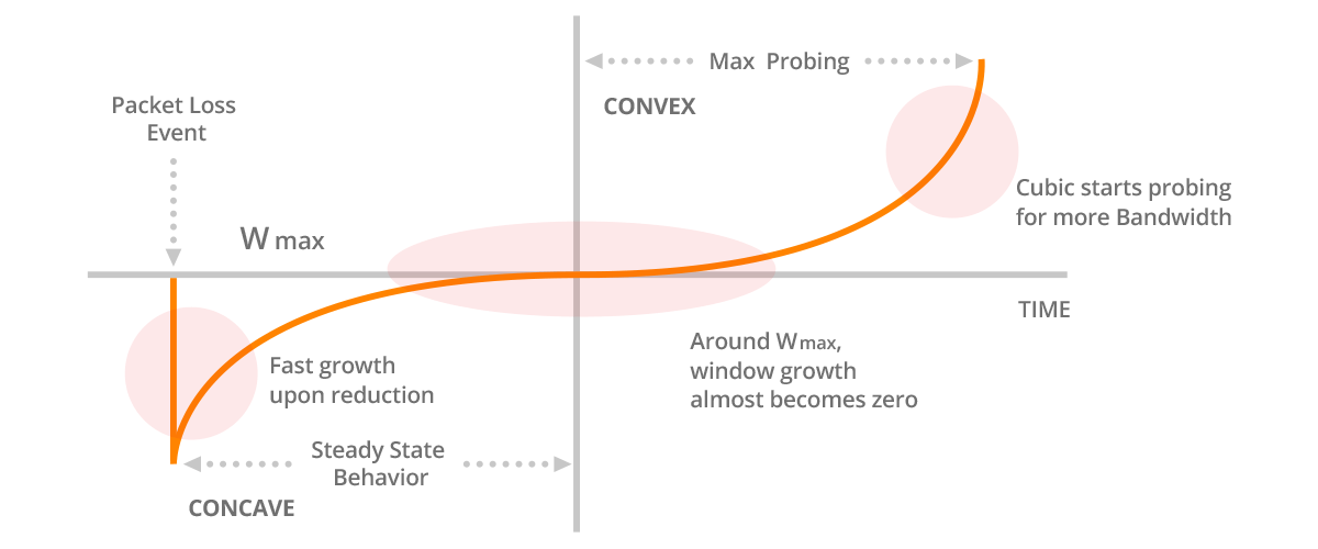
Where as the traditional TCP Reno congestion control was simple and intuitive to understand, CUBIC takes more digesting. The exact algorithm is described in the afore-mentioned paper, and here is a short summary. At the core of the algorithm, there is $W_{max}$, the window size when last loss event (packet loss or ECN mark) was observed. Like traditional TCP congestion control, CUBIC maintains congestion window (cwnd) that determines how many unacknowledged packets can be sent to the network. When cwnd is less than $W_{max}$, CUBIC is in the Concave region, where it increases the window first more aggressively, but as cwnd starts to approach $W_{max}$, the window increases more slowly following a cubic function defined in the algorithm. If cwnd exceeds $W_{max}$, CUBIC is in Convex region, and starts to increase the window size faster, as the current cwnd takes distance to the previous sample of $W_{max}$.

The idea of CUBIC is to try to probe fast the proper network capacity, but once found, keep the transmission rate steadily there. On the other hand, the network state can change at any time, for example, if other traffic source goes away from a bottleneck resource. In such case CUBIC tries to find the new, improved network capacity as efficiently as possible.

The below picture is taken from network article by Noction, that illustrates the above described dynamics of the CUBIC algorithm.

Delay-based algorithms

Delay based congestion control algorithms (e.g. DUAL, different variants of Vegas, FAST) are based on measuring the round-trip time of data transfer and aim to estimate based on the delay variation whether there is congestion at the bottleneck link. The minimum measurement of round-trip time indicates the ideal state when there is no queue at the bottleneck link. When measured round-trip time starts to increase, that is taken as an indication that queue is starting to build up and the transmission rate should therefore be reduced.

Delay-based algorithms are not in wide-spread use. One problem is that they don’t co-exist well with the traditional loss-based algorithm, and in some situations can unfairly gain the bandwidth from flows that are using loss-based algorithm.

Model-based congestion control

To address the challenges of loss-based congestion control, i.e., the tendency to increase network buffering and slow reaction to congestion, Google developed a different approach for congestion control that is not solely based on observing losses or ECN marks, called BBR. It takes quite different approach to congestion control: it aims to measure the bandwidth and delay of connection path (excluding delays caused by buffering) and adapt the transmission rate to that so that there would be no queues accumulating at any router.

The below graph illustrates the dynamics of how increasing the amount of unacknowledged data in transit affects the experienced delay and data delivery rate. In the context of network buffering we already discussed similar graph, this closely follows the illustration in the BBR paper.

The product of bottleneck bandwidth and round-trip delay of the connection path (i.e., Bandwidth-delay product, BDP) determines the ideal transmission rate for the given connection: if a transport protocol sends at lower speed, we do not achieve the full delivery rate, but round-trip time is as short as it can be, as defined by physics. There are many applications that simply do not have much data to transmit and they operate in this space (we call transmission to be “application limited” in such case), regardless of chosen congestion control algorithm.

When transmission rate increases beyond bottleneck BDP, the packets start to accumulate into network queues and buffers (being “bandwidth limited”). As discussed before, this starts to increase the experienced end-to-end delay, but does not improve delivery rate, so this has negative effect on observed performance. When buffers get full, packets start to get dropped, and only then the traditional loss-based congestion control algorithm starts to react (or one RTT later, to be exact). Of course active queue management helps a bit, adding some packet losses already in the bandwidth-limited phase.

BBR aims to estimate the current bottleneck bandwidth by measuring the delivery time of packets from incoming acknowledgments, and including the measured round-trip delay into estimation. The algorithm needs to estimate when the sender is application limited and when bandwidth limited to be able to collect accurate measurements. On the sending side, transmission of packets is paced, i.e. controlled by timer so that they are sent exactly at the rate of estimated bottleneck bandwidth. For a more detailed description, you can start from the BBR paper and then for additional details, refer to an Internet-draft that is to become Experimental RFC at some point.

Ideally, when everything works perfectly, this should avoid queues from forming up. Unfortunately, the Internet does not work perfectly: the network conditions change all the time based on other users of the network: there are different applications and different protocol stacks implementing different congestion control algorithms. In addition, there may be badly behaving users that may try to collapse the network performance intentionally. BBR is still considered experimental, and not a default algorithm, e.g. in Linux, but many datacenter operators such as Google and Cloudflare are known to use it already in production.

Congestion control

Traditional congestion control

Further reading

Network buffering and latency

Further reading

Active Queue Management

Random Early Detection (RED)

Controlled Delay (CoDel)

Flow Queue CoDel (FQ-CoDel)

Linux implementation

Further reading

Explicit Congestion Notification (ECN)

Setting up ECN in Linux

Classes of Modern congestion control

Loss-based algorithms

Delay-based algorithms

Model-based congestion control

Further reading